Figure 2.2)
Each degree of freedom denotes an independent way in which a body can move. A completely free body has six degrees of freedom. Given standard rectangular coordinates, a free body can translate in any of the three coordinate directions and it can rotate around the three coordinate directions.
PA makes use of the degree of freedom limitations on bicycle components. For example, in the reference frame of the ground, a dual suspension bicycle main triangle has three relevant degrees of freedom while the bike is traveling in a straight line. It can translate horizontally and vertically, and it can rotate, all in the plane defined by the rear wheel. The balance of the rider limits the other degrees of freedom. If we fix the main triangle in space, relevant bicycle components only have at most one degree of freedom.
C) Nature Varies Smoothly (NVS).
The equations describing the laws of nature are continuous relations (usually stated as functions). The value on one side will not jump discontinuously as the parameters on the other side vary continuously.
(This excluding the quantum realm - very small, very big, very cold, etc.)
As a result, if we imagine a pivot position varying smoothly along some arm in a mechanism, the equations of motion will vary smoothly also. That is, the physical situation (laws) will not jump at some point. The way the mechanism behaves will change continuously.
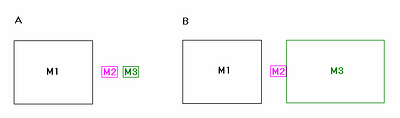
One of the most difficult things physics students have to grasp is when and how to make approximations. The simplest form of approximation is that involving quantities much larger or smaller then other relevant quantities in a given physical situation. We will give two examples of proper and improper approximations by this method, using mass.
Consider the mass M1 which is much, much bigger then the non-zero masses M2 and M3 in Figure 2.2 A). The masses move without friction in one dimension. In considering the motions of all bodies, approximating M2 and M3 as having zero mass would not be useful, since information about the interactions of the small bodies would be eliminated. On the other hand, if we approximate M1 as infinite, useful calculations may still be done (this is often done when considering human-sized objects interacting on the earth).
In Figure 2.2 B), we have the opposite situation from Figure 2.2 A). Here, we might very well neglect the mass of M2 in quantifying the results of M1 colliding with both M2 and M3.
These two examples show that, in certain situations, the odd entity may be approximated.
Figure 2.2)
Next, consider Figure 2.3 A), which depicts a block of mass M connected by a rope to a suspended wheel that is of very small mass relative to the block and spins with negligible friction. If we want to quantify what happens when the block is suddenly dropped, we could not ignore the mass of the wheel, since our approximations would then describe a non-physical situation namely the unconstrained angular acceleration of a zero-mass body. On the other hand, if we were to ask the angular acceleration of the wheel in the Atwood device in Figure 2.3 B), we could get a pretty good answer while ignoring the mass of the wheel, if both M and m are large compared to the wheel.
For a further discussion of this topic, see the Mass Approximation. section in P.A. Basics.
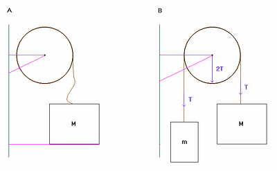
Figure 2.3)